
If you had a million years on this Earth, you might find time to read every possible research paper on energy modelling and come up with a pretty good understanding of window and door behaviour. But having spent nearly 30 years in this field, nothing has gotten any simpler. The closer you look, the more there is to consider. But sometimes we just need a basic placeholder number instead of nothing. Yes, windows are complex because our planet keeps spinning around while it orbits a Sun, and windows might face different directions and may even be at different angles, but in a lot of cases, windows are generally vertical, and are also often evenly distributed across elevations – just look at any condo tower – who wants the unit with no windows?
That’s why we seized on an idea by Dr. Ted Kesik to develop a simpler metric for window behaviour in early schematic design. Disclaimer: this approach may be considered blasphemy to the energy modelling community. But, in early Schematic Design, we don’t use energy modellers, and Architects and Designers need simpler tools to understand loads generally, and that is why we’re ‘inventing’ a way of doing this as a placeholder, until we have a more developed building design, and a more delineated BEM (Building Energy Model).
In a heating climate, where heating loads are bigger than cooling loads, windows generally lose more energy than they gain. Until you start designing high performance envelopes – then windows can start gaining more energy than they lose. You may have seen those window energy balance diagrams with a bunch of arrows doing different things to and through windows. Some energy transmitted, some reflected, some spins around in the window like a pinball for a bit, etc. Here’s what we mean:

We’re not going to get into all of that – the dynamic/hourly energy model does this for us – we just want to isolate a result for Ontario we can use as an average for gains per unit area. Typically windows are modelled in 8 different cardinal orientations, N, E, S, W and NE, SE, SW, NW. What if we don’t yet know window orientations or sizes, but we wanted to account simply for gains and losses of any window on an envelope, on a per square meter basis? Well, knowing what the window loses, in terms of energy, is easy; it’s a function of it’s U-value, or the rate at which it transmits radiant* energy from a hot place to a cold place – in a heating climate that means from inside to outside. But how much solar energy is transmitted from the cold place to the heated place – basically the reverse but through direct radiation (SHGC notwithstanding) – when it’s a sunny day outside? (*thermal gains and losses are handled separately from radiant gains and losses in OBJECTIVE).
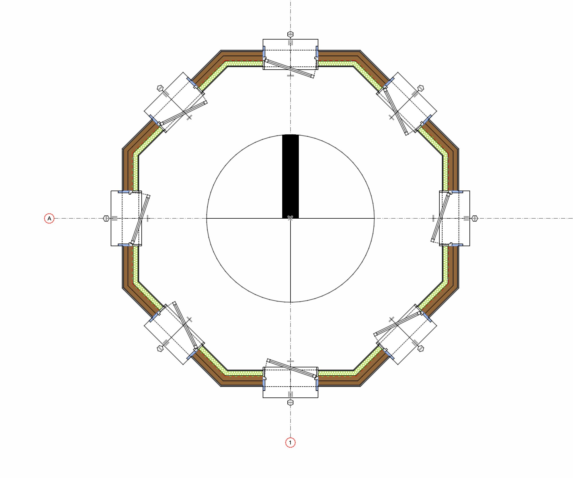
Well, if we make a tiny test building in the shape of an Octagon: with a pretty good 1m2 window of our favourite brand and spec (casement, triple glazed, low-e, nonconductive spacers, with a moderate SHGC and DST of about 40%, and a U-value of about 1.3, and about 70% of the window is glass, the rest is frame area, etc.) and put this thing in Toronto (location matters, as a function of latitude more than anything else, but also typical cloud cover) – how much energy do we gain over the course of a year? We run the dynamic simulation in ArchiCad’s EcoDesigner (Which uses StruSoft’s VIPCore engine, a Swedish dynamic modelling engine).

Here’s what we get: 1,096.8 kWh/yr. So, if we divide that by our 8 windows, we get an average for solar heat gain of 137.1 kWh/m2. We can use that as a ‘Solar Gain Load’. So if our building has 10m2 of windows, equally applied to 4 key elevations, we should expect 1,371 kWh/m2 gained in a year. If we have 1,000m2 of windows, 137,100 kWh per year, etc. Now – this gain is often when we don’t want it – in the Summer or cooling season.

One way we can smush these gains is to provide 100% physical shading (not to be confused with SHGC, a function of the glass itself) of windows in the cooling season, that means side fins and top fins or louvres or rolling shutters. Physical shading devices that are outside of the glazed surfaces. Then we can just look at the Heating Season gains as a contribution when we want it and not a needless cooling load we don’t want in the Summer. The ‘Heating Season’ in Canada is generally considered to be from Oct 1 to April 1. So let’s look at just that as a period for useful solar gains – which is the ultimate purpose of this exercise. Only 378 kWh (the sum of my Heating Season Gains by Month in the table below) of our 1,096.8 kWh total annual gains are useful, because they take place when we are heating the building. Solar gains in Spring and Fall are another matter, and we can generally dump most of them by opening a window, just as if we can unzip our jacket if we are feeling too warm. Solar gains in the Summer are a problem, especially when humidity makes opening windows impractical, but that is another topic on the ‘Latent Load’ and how much ‘Free Cooling’ is available to us through open windows and/or ventilation – more on that in the Cooling discussions, but to simplify the discussion for now, let’s assume we’re all good designers and have planned for physical shading structures, fins, louvres or some other method to eliminate direct solar gains in the cooling season by 100%, then we don’t need to figure out what to do with them, they simply don’t make it inside the building!

So with heating season solar gains is effectively bumped down to 378/8, we get 47.25kWh/m2•yr. So if we have 1,000m2 of windows, we can count on 47,250 kWh of useful gains in the Winter or heating season. Easy enough right? That’s what we’re going to run with for our Schematic loads, for a generic, 1m2 window of decent quality – that is blind to orientation but has 100% cooling season shading!


But how reliable is this 47.25kWh/m2 – does this number reproduce in other modelling software? Well, our colleague Ben Frost in New Zealand just used DesignPH to test the assumption using a standard PHPP window, in Toronto, at 0m ASL, and while his were larger, the result tracks with our own values, Ben gets 52.41kWh/m2. The small difference could be from the fact that our smaller windows with deeper frames offer more self-shading of the glass components, but what this does is validate that ~50kWh/m2/yr generally works as a gains placeholder for SD stage modelling. PS – If your windows are facing North, they gain 0kWh/m2, but the other elevations make up for this loss with 80, 70, 30, etc – which is how we arrive at our global average.

Stay tuned to find out how we use these values in early stage energy-model massing using simple slab objects and ArchiCad supercharged properties and expressions next! Thanks again to Dr. Kesik for a simple idea we will deploy right away!
Addition: 2024.10.02; Students at McGill’s School of Architecture were asking how to plan for orientation specific design of facades since the Montreal street grid is about 45ºCW of a N,E,S,W orientation. Well, since we have all 8 key cardinal values from this Octagone dynamic hourly model, let’s explore this next. So we added the G.2.5 Rotate Model switch, to help when urban grids like Montreal are not aligned with N, E, S, W but are rather 45º to this orientation, clockwise or counter-clockwise, there are three toggles, 0º, 45ºCW, 45ºCCW. Why not a range of angles? Well, because our Octagone model only handles the 8 cardinal orientations, and furthermore, we start splitting hairs at this point. What we’ve found is most buildings ‘benefit’ from the ‘average’ method over the orientation-specific method of accounting for solar gains. What the G.2.5 Rotate Model switch does when you rotate 45ºCW, is simply apply the NE gains to the N windows, the SE gains to the E windows, the SW gains to the South windows, and the NW gains to the W windows. Is there a big difference in the values? Not as much as you might think. There are a few reasons for this, but windows placed halfway into a wall tend to ‘self-shade’ themselves, so there is a very narrow period in the year when they are not shaded at the top or sides by the geometry of the wall itself, maybe only an hour of any given day! And furthermore, more solar energy enters when it is at 90º to the surface of the window or the incident angle. We get closer to this incident angle in the morning and afternoon when the sun is low in the sky, but less when it is higher in the sky (ie. ‘high‘ noon). So even though the total solar intensity arriving inside the building is greater during the cooling season, we tend to want to shade that out either with physical shading devices, which the user defines at G.2.8 Shading Cooling Season in the case of physical shading devices, or with G.2.1 Solar Gains Heating Season Intensity, where we can apply a window film which reduces solar transmission known as the SHGC or ‘Solar Heat Gain Coefficient‘, the higher the number, the greater the solar transmission. If you can rely on very good physical shading systems, you can set that number higher, like 0.6 (60%), but if your client doesn’t have a budget for shading systems, then a lower transmission value like 0.35 (35%) will help reduce your total cooling load. You can play around with these variables to determine how you can get the lowest possible TEUI score, as a combination of SHGC, Shading and Orientation. G.2.7. Solar Gains Cooling Season By NESW does not yet use the Rotate Model switch – but that is on the roadmap to add it.
For those of you that want more detail, here are the annual values for all 8 cardinal orientations as Annual Integrated Direct Radiation in kWh/m2/yr:
- North: 1.31
- Northeast: 34.69
- East: 76.94
- Southeast: 86.59
- South: 70.74
- Southwest: 60.4
- West: 25.86
- Northwest: 2.88
Average = 44.92 kWh/m2/yr (note: this is different than solar gains useful to us in the heating season calculated above as this number considers the full year of ‘integrated’ or used gains, whereas our previous gains number only looked at Jan-Mar and Oct-Dec gains, which we defined as the ‘Heating Season’). These values are built in to the equation on line 105, which looks like this:
=IF(I105="0º",((D70*1*D$102/0.5)+(D71*75*D$102/0.5)+(D72*70*D$102/0.5)+(D73*25*D$102/0.5))*(1-G108),IF(I105="45ºCW",((D70*34.69*D$102/0.5)+(D71*86.59*D$102/0.5)+(D72*60.4*D$102/0.5)+(D73*2.88*D$102/0.5))*(1-G108),((D70*2.88*D$102/0.5)+(D71*34.69*D$102/0.5)+(D72*86.59*D$102/0.5)+(D73*60.4*D$102/0.5))*(1-G108)))

!!! Where D70 = Windows North, D71 = Windows East, D72 = Windows South and D73 = Windows West. 
Edit: We have now finalized behaviour, rotations can be applied to any Window line, rather than the whole building, because the orientation of opaque assemblies doesn’t factor in to OBJECTIVE modelling.
Leave a Reply